Transiting Planets
Using another very clever technique, we can not only discover extrasolar planets, but determine fairly accurately how big they are and, armed with Kepler’s Third Law, we can find out how far they are from the star.
At this point show an orrery (model star with planets) with a light sensor aimed at it and a computer display of the light sensor output to generate a transit light curve.

You can do this either as a live demonstration or show two side-by-side movies of the demonstration.

The example we use here is for the “Walking Orrery” (item 3A in the Materials section):

Make sure the light sensor is aimed at exactly at the model star (light). Enable the system you have prepared to project data from the light sensor as a Brightness vs. Time graph on the dome. Caution the audience that you are about to turn on a model star, then turn on the model star, but do not spin it yet.

Point out to the audience the light sensor, model star (light) and planet(s). Explain that the light sensor measures the brightness of the star and will feed star brightness data to a computer and show us a graph of brightness changes.

Vary the display in an obvious way—by putting your fingers or hand between the sensor and the light.
The light sensor also called a photometer because it measures how many photons of light are going into it. That picture [point to graph display on the dome] shows the brightness of the star! It’s a graph of light brightness—called a light curve. You can even tell how long my hand is blocking the light without even being able to see my hand. Just look at the light curve….
Have audience volunteers block the light with their hands.

Let the graph stabilize so the audience can see the flat line that represents the normal star’s brightness, as detected by our “telescope” sensor.

Then point out the orrery again and explain:
“This is a model star and this a model planet.”

Run the orrery by having a volunteer holding the planet walk around a volunteer holding the star (for Walking Orrery)

If using any of the other orreries (B through D) turn the crank on the orrery so the planet periodically blocks the light entering the sensor, making a light-curve graph. If a volunteer is helping, instruct them to crank gently and steadily. If the volunteer is somewhat erratic, you can comment that it looks like our solar system machinery is “only human.”
What happens when this extrasolar planet passes between the star and our photometer?
[There is a dip in the graph.]
The extrasolar planet is blocking the light from the star, and our sensor detects it!
What a great way to find extrasolar planets!
It’s like an eclipse.
Astronomers call it a “transit,” which means “going across.”
Looking for stars that are having their light blocked by a planet going in front is called the “Transit Method” of finding extrasolar planets.
One limitation of the Transit Method is that it only works if the extrasolar planet and its star are tipped just the right way.
What if the extrasolar planet orbited the star at an angle that was not lined up with our sensor?
[No transit could be detected.]
Optional video: showing how transits can only be seen when we are viewing from sideways to the orbit.
Let’s see what we can tell from this light curve graph.
Have volunteers again run the Walking Orrery—one holding the star still and the other walking around it with the planet. [If using another orrery, have a volunteer crank the orrery.]
How can you tell from the light curve if a planet is big or small?
[Big planets make deeper dips in brightness.]
We can also measure how often light is blocked—that means how much time passes from here to here on the graph.
Point out the distance between dips on the projected graph.
We saw this before, too! That’s the period of the orbiting planet.
How can you tell from the light curve if the planet is close to or far away from its star?
[Farther out planets make dips that are more widely spaced.]
With the Walking Orrery you can have two planet volunteers each with a different sized planet mounted on a pole and walking around (orbit) the star at different speeds. The one closer to the star should walk faster (bigger steps) than the one farther from the star.

If space is limited you can have one planet orbiting at a time, each for about 15 to 20 seconds, one after the other. This produces two light curves side by side, each one 15–20 sec long. In some ways, this is even easier for people to analyze than the light curve with two planets going simultaneously.

With 1-planet portable model, you can similarly generate separate side-by-side light curves by stopping after 15 or 20 seconds, for a quick switch of planets. That also generates two “half” light curves, side by side.
If the dips on the light curve graph are close together—then the planet is orbiting the star really fast, and it must be really close to the star. That means it is a hot planet.
Look how close the dips are in that light curve graph!
[Point to most closely spaced dips.]
That’s a close, hot planet!
[Point to most widely spaced dips.]
Then the planet would have to be far away from the star, and that means it is a colder planet. Look how far apart the dips are on that light curve graph! That planet is really creeping—must be far from its star. Brrr! That’s a cold planet!
Since big planets block a lot of light and small planets only block a little bit of light, big planets are easier to find than small planets! Just like with the spectra of star wobbles. Big hot Jupiters are the easiest to find.
ALTERNATIVE TO LIVE DEMONSTRATION

VISUAL: Orrery

If you not to do a live demonstration, use the Orrery and Light-Curve-Graph movies.

Shown here is a 7 second video of a 3-planet orrery model.
VISUALS (pair of alternative movies): The orrery in action synchronized with the live light curve graph

Show these movies side by side or one above the other, and run them synchronized.

This movie (sp22bLiveGraph-Orrery) is 32 seconds of the 3-planet orrery being cranked.
This is the matching movie (sp22cLiveGraph-Orrery) of the graph being formed as the orrery operates.
VISUAL 18 (movie): Transit Light Curve
(sp29bOSNanimkurz.mp4)
This movie shows a light curve generated by a real transit observing telescope. Above it is an artist’s representation of what the planet would look like transiting the star, but size of the planet is exaggerated—extra large.
From detection, astronomers generate a light curve, and measure the dimming effect.
From the small change in brightness, you can figure out the size of the planet.
If you see a big drop, what does that tell you about the size of the planet?
[It must be a big planet.]
Right—and a small drop means a small planet.
Optional
DIGITAL EFFECT: Transit of Earth
If your digital system can show it, display a rendering of Earth passing in front of the Sun and explain:

“To a distant astronomer, here’s what a transit of Earth might look like. Earth passes in front of the Sun, and then one period later—that is, one year, in Earth’s case—you get another transit.“
VISUAL 19 (movie): Optic Path
In the case of Kepler, we’re looking at distant stars. Planets pass in front of their stars, and then the instruments on Kepler detect that change in brightness.

Kepler had to stare long enough to see the planet repeat the transit several times. From the period of the transits and using Kepler’s Laws of planetary motion, you can calculate how far the planet is from its parent star and know if it is in the habitable zone.
VISUAL 20 (still): Kepler spacecraft
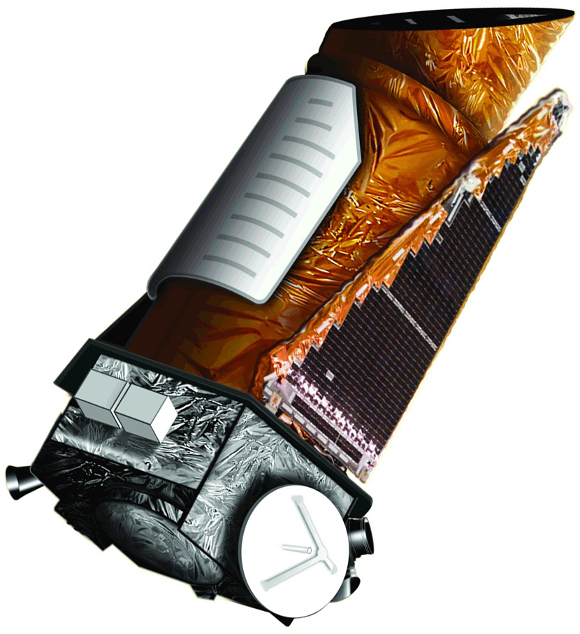
We can think of the light sensor we were using as a model of the NASA Kepler spacecraft and its light sensing camera. The Kepler instrument used a light sensor like the one we’ve been using today, except that it’s huge, with nearly 100 million pixels, and it’s in a big telescope to collect lots of light. How many pixels does your digital camera have? 5 megapixels? 8 megapixels? I bet it’s not 100 megapixels, like the Kepler spacecraft camera! And with that sensitivity, Kepler can generate a light curve for individual stars to find planets!
The transit method of planet finding is second only to the spectroscopic method in terms of numbers of planets discovered so far, but the Kepler Mission could change all that. In February of 2011, the Kepler team released data containing 1,235 planet candidates. The planet candidates are not all confirmed planets, but many of them are very likely real planets.